Introduction

For the CSCE 489 final project, I built a marble labyrinth simulation that uses device motion (tilting) as inputs to move the marble throughout the map. Reasonably accurate physics are implemented, along with a few interpolation techniques to improve the appearance of motion.

The code is written in Swift, using Metal for rendering and some computation. Physics is simulated using symplectic Euler, and interpolated between frames using linear interpolation.

Input

Input to the simulation is accomplished by tilting the device; specifically, the roll and pitch axes of the device are scaled to produce the angle vector \(\theta_{device}\) which is in turn used as an input to the physics simulation.

These updates are delivered asynchronously at around 30Hz from the CoreMotion framework. While it is possible to request faster updates, I found that data was much noisier above this speed. It also made masking the computation time for the physics calculation, since the physics simulation could run completely decoupled from the rendering loop.

In other words, the rate of the physics simulation is directly proportional to the rate at which accelerometer data is received.

Physics

The simulation handles two types of bodies: dynamic (ones that move/are affected by forces) and static (immovable objects, such as walls or floor.) The primary difference between the two is that static objects do not get integrated changes to their positions. This is particularly useful for walls, which are fixed, but still impart a certain force on the marble when it collides with one so that it bounces.

Each step of the physics simulation, the device angles \(\theta_{device}\) are multiplied by some constants \(\vec{C}\) and used to modulate the global gravity vector's effect on the marble. This, in turn, causes it to roll as the device is tilted: the force applied to the marble is \(\vec{F}_{rolling} = \vec{C} \times \theta_{device} \times \vec{g}\).

No other objects are affected by the rotation of the device. A light source is placed directly above the marble and tracks it, both translationally and rotationally, and thus gives the illusion that the rest of the map is moving. This means that during display, we have to only use translations, which simplifies things a little bit.

Collisions

After integrating velocities and positions, the marble's \(\vec{x}\) is checked to see if it collided with a spring, end goal, or wall. This is done by checking whether the distance between the center of the marble and any potential intersection surfaces is less than the marble's radius.

In the case of walls or floors, most of the marble's velocity is absorbed, while a small proportion of it is kept and set in the opposite (normal) direction of the previous velocity. For springs, a constant impulse is applied to the marble, at the normal angle to where it hit the spring.

Since it's possible for the marble to fall off the map (thanks to springs,) there's a small check that places the marble back at its starting position when it's at a minimum \(5r\) units below the nearest collidable object. Limiting this check to being below the object allows the marble to fly far above the map, while triggering only once it's fallen off.

I experimented with casting a ray between the old and new position of the marble, and checking whether this ray intersected with any objects to detect collisions. This approach has the benefit of reducing the chance that the marble might clip through solid objects if moving particularly fast; however, it was much more difficult to implement properly and efficiently. I adjusted the device angle force constants instead to reduce the maximum velocity of the marble to mask this issue.

Interpolation

Since the physics simulation runs at only 30Hz, yet we render at up to 120 Hz (fps), some interpolation is necessary to ensure the appearance of smooth, continuous motion.

To accomplish this, linear interpolation between \(\vec{x}_{marble}\) and the previous frame's position is performed on every physics update step. This means that the rendered image can be up to 4 frames out of date; but at 120fps rendering, this causes no problem with making the interactions believable.

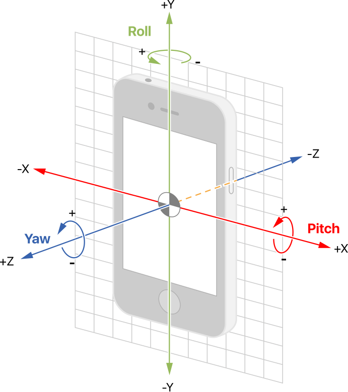
Particle System

Lastly, a particle system was implemented to indicate that you've reached the goal of the map. This takes the form of a bunch of solid billboarded quads that vary in saturation and alpha component as they're created.

Computation for the particle system takes place on the GPU through a compute shader. This shader takes as an input, as an uniform, a struct containing the parameters of the particle system: the gravity vector \(g\), particle mass \(m\), dampening factor \(d\), its life span, and various deltas for initial velocity \(v\), color, etc. At each frame, the compute shader is invoked and generates vertex data (for quads) in an output buffer.

First, the forces acting on the particle are accumulated: \[\vec{f} = m\vec{g} - d\vec{v}\] Using symplectic Euler, given the time since the last step in seconds, \(h\), we can integrate the velocity and position of each particle: \[\vec{v} = \vec{v}_{prev} + \frac{h}{m}\vec{f}\] \[\vec{x} = \vec{x}_{prev} + h\vec{v} \]

Since we need access to the previous per-particle velocities and positions, we keep a second buffer that contains this data from the previous invocation. There's no collision with the floor (or other objects) so the initial velocity is set high enough that particles will never live long enough to fall downwards.

Particles are drawn as solid colored quads, with alpha blending, after the rest of the scene has been drawn. They do not participate in the physics simulation.

Map Data

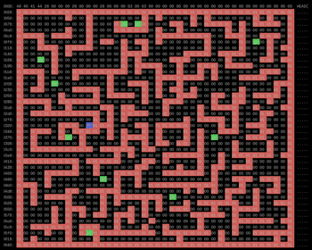
The layout of the level is read from a fixed binary file included with the program; this data is then processed into the actual geometry for the walls, and used in physics simulation to determine where the walls are located.

At its core, the file is essentially a 2D array, where each byte corresponds to one 'tile' of the map. Various different byte values indicate different items at that position: for example, 0x01 is a wall, while 0xFF is the end goal. A small header at the start of the file specifies the size of the map, as well as the starting location of the marble.

Primarily, the choice of a binary format was driven by how easy it is to parse; likewise, hex editors make relatively decent level editors.

References

Below is a list of various resources I consulted while working on this project.

• Metal by Example: Many useful resources consulted while building the rendering engine.
• Accelerate.framework reference: This framework contains lots of fun math-y routines, including functionality similar to Eigen. This is used for the physics simulation.
• Class assignments and Labs: Many previous assignments and optional labs were used as inspiration/to understand the basic algorithms. Swift and C++ are similar enough that I was able to translate the code I had written for previous assignments for many components.